Geolocation Functions

Shareloc has several main functions:

Localization
Triangulation
Rectification Grid Computation

Examples can be found in tests directory of Shareloc source code.

Localization

Localization means mapping between image coordinates and ground ones using geometric model.

Localization functions can be called via its class or directly using geometric models. It can be simplified as the intersection of a LOS and the terrain.

Following information are needed for localization functions:

a geometric model

elevation information, details in Elevation handling section.

image information in order to use geotransform, details in Conventions section.

EPSG code to specify ground coordinate system

shareloc.geofunctions.localization.Localization class collect these data to set up the localization functions. It is possible to use geometric model directly using shareloc.grid.Grid and shareloc.rpc.rpc.RPC for advanced used.

class Localization:
"""base class for localization function.
Underlying model can be both multi layer localization grids or RPCs models
"""

def __init__(self, model, elevation=None, image=None, epsg=None):
    """
    constructor
    :param model : geometric model
    :type model  : GeoModelTemplate
    :param elevation  : dtm or default elevation over ellipsoid if None elevation is set to 0
    :type elevation  : shareloc.dtm or float or np.ndarray
    :param image  : image class to handle geotransform
    :type image  : shareloc.image.Image
    :param epsg  : coordinate system of world points, if None model coordinate system will be used
    :type epsg  : int
    """

Direct Localization

Direct localization returns ground coordinates $(\lambda,\phi,h)$ for image position (row, column) $(\lambda,\phi) = direct\_localization(row,column)$ .

$h$ can be explicitly set as input (in case of constant altitude over ellipsoid) : $(\lambda,\phi,h) = direct\_localization(row,column,h)$ , or found via the underlying DEM : $(\lambda,\phi) = direct\_localization(row,column)$

$(\lambda,\phi)$ can be geographic (lat,lon) or cartographic depending on the chosen CRS

def direct(self, row, col, h=None, using_geotransform=False):
    """
    direct localization

    :param row: sensor row
    :type row: float or 1D np.ndarray
    :param col: sensor col
    :type col: float or 1D np.ndarray
    :param h: altitude, if none DTM is used
    :type h: float or 1D np.ndarray
    :param using_geotransform: using_geotransform
    :type using_geotransform: boolean
    :return coordinates: [lon,lat,h] (2D np.array)
    :rtype: np.ndarray of 2D dimension
    """

Inverse Localization

inverse localization returns image position (row,column) for ground coordinates $(\lambda,\phi,h)$ $(row,col) = inverse\_localization(\lambda,\phi,h)$ .

def inverse(self, lon, lat, h=None, using_geotransform=False):
    """
    inverse localization

    :param lat:  latitude (or y)
    :param lon: longitude (or x)
    :param h: altitude
    :param using_geotransform: using_geotransform
    :type using_geotransform: boolean
    :return: coordinates [row,col,h] (1D np.ndarray)
    :rtype: Tuple(1D np.ndarray row position, 1D np.ndarray col position, 1D np.ndarray alt)
    """

Colocalization

colocalization returns image positions (row2,col2) in image 2 from (row1,col1) position in image 1

def coloc(model1, model2, row, col, elevation=None, image1=None, image2=None, using_geotransform=False):
    """
    Colocalization : direct localization with model1, then inverse localization with model2

    :param model1: geometric model 1
    :type model1: GeomodelTemplate
    :param model2: geometric model 2
    :type model2: GeomodelTemplate
    :param row: sensor row
    :type row: int or 1D numpy array
    :param col: sensor col
    :type col: int or 1D numpy array
    :param elevation: elevation
    :type elevation: shareloc.dtm or float or 1D numpy array
    :param image1  : image class to handle geotransform
    :type image1  : shareloc.image.Image
    :param image2  : image class to handle geotransform
    :type image2  : shareloc.image.Image
    :param using_geotransform: using_geotransform
    :type using_geotransform : boolean
    :return: Corresponding sensor position [row, col, True] in the geometric model 2
    :rtype : Tuple(1D np.array row position, 1D np.array col position, 1D np.array True)
    """

Triangulation

Triangulation gives 3D intersections between LOS coming from 2 geometric models.

Triangulation is calculated according to the following formula:

$x= \left(\sum_i I-\hat v_i \hat v_i^\top\right)^{-1} \left(\sum_i (I-\hat v_i \hat v_i^\top) s_i\right)$

where $v_i$ is the orientation of the LOS i and $s_i$ the hat of the LOS i

def sensor_triangulation(
    matches,
    geometrical_model_left,
    geometrical_model_right,
    left_min_max=None,
    right_min_max=None,
    residues=False,
    fill_nan=False,
):
    """
    triangulation in sensor geometry

    according to the formula:
    .. math::
        x =
        \\left(\\sum_i I-\\hat v_i \\hat v_i^\\top\\right)^{-1} \\left(\\sum_i (I-\\hat v_i \\hat v_i^\\top) s_i\\right)
    Delvit J.M. et al. "The geometric supersite of Salon de Provence", ISPRS Congress Paris, 2006.


    :param matches :  matches in sensor coordinates Nx[row (left), col (left), row (right), col (right)]
    :type matches : np.array
    :param geometrical_model_left : left image geometrical model
    :type geometrical_model_left : GeomodelTemplate
    :param geometrical_model_right : right image geometrical model
    :type geometrical_model_right : GeomodelTemplate
    :param left_min_max : left min/max for los creation, if None model min/max will be used
    :type left_min_max : list
    :param right_min_max : right min/max for los creation, if None model min/max will be used
    :type right_min_max : list
    :param residues : calculates residues (distance in meters between los and 3D points)
    :type residues : boolean
    :param fill_nan : fill numpy.nan values with lon and lat offset if true (same as OTB/OSSIM), nan is returned
        otherwise
    :type fill_nan : boolean
    :return intersections in cartesian crs, intersections in wgs84 crs and optionnaly residues
    :rtype (numpy.array,numpy,array,numpy.array)
    """

References :

Delvit J.M. et al. The geometric supersite of Salon de Provence, ISPRS Congress Paris, 2006. (http://isprs.free.fr/documents/Papers/T11-50.pdf)

Rectification Grid Computation

Rectification or stereo-rectification refers to the image transformation in epipolar geometry.

A rectification grid is a displacement grid used to resample sensor gemetry to epipolar one. Shareloc rectification grids respects OTB convention for displacement grids.

To generate the images in epipolar geometry from the grids computed by shareloc and the original images, one can refer to the Orfeo Toolbox documentation here . Algorithm details can be found in reference below.

def compute_stereorectification_epipolar_grids(
    left_im: Image,
    geom_model_left: GeoModelTemplate,
    right_im: Image,
    geom_model_right: GeoModelTemplate,
    elevation: Union[float, DTMIntersection] = 0.0,
    epi_step: float = 1.0,
    elevation_offset: float = 50.0,
) -> Tuple[np.ndarray, np.ndarray, int, int, float, Affine]:
    """
    Compute stereo-rectification epipolar grids. Rectification scheme is composed of :
    - rectification grid initialisation
    - compute first grid row (one vertical strip by moving along rows)
    - compute all columns (one horizontal strip along columns)
    - transform position to displacement grid

    :param left_im: left image
    :type left_im: shareloc Image object
    :param geom_model_left: geometric model of the left image
    :type geom_model_left: GeoModelTemplate
    :param right_im: right image
    :type right_im: shareloc Image object
    :param geom_model_right: geometric model of the right image
    :type geom_model_right: GeoModelTemplate
    :param elevation: elevation
    :type elevation: DTMIntersection or float
    :param epi_step: epipolar step
    :type epi_step: float
    :param elevation_offset: elevation difference used to estimate the local tangent
    :type elevation_offset: float
    :return:
        Returns a Tuple containing :
            - left epipolar grid, np.ndarray object with size (nb_rows,nb_cols,3):
                [nb rows, nb cols, [row displacement, col displacement, alt]]
            - right epipolar grid, np.ndarray object convention (nb_rows,nb_cols,3)
                [nb rows, nb cols, [row displacement, col displacement, alt]]
            - number of rows of the epipolar image, int
            - number of columns of the epipolar image, int
            - mean value of the baseline to sensor altitude ratio, float
            - epipolar grid geotransform, Affine
    :rtype: Tuple
    """

Epipolar grid generation adapted for parallel computing

We generate the left grid point by point, and for each point on the left grid, we compute its equivalent on the right grid using the colocalization function. Therefore, in the following sections, we will only focus on describing the process of generating the left grid.

The algorithm follows these broad guidelines:

1.Calculation of the top-left corner of the grid is performed using the init_inputs_rectification function.

2.Starting from this first point, we compute the first columns of the grid.*compute_strip_of_epipolar_grid(axis=0)*

3.Computation of each row, by stride, from the first columns.*compute_strip_of_epipolar_grid(axis=1)*

To calculate the next point from the current one, we follow these steps:

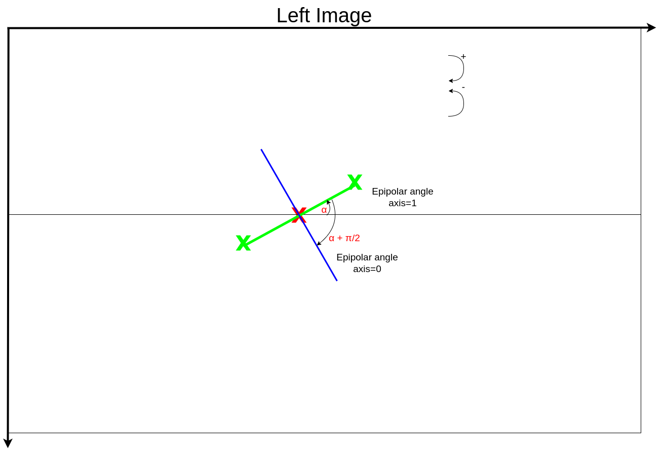
1.Obtain the local epipolar line: We perform colocalization on the current left grid point to obtain its corresponding point on the right image. Then, we conduct another colocalization back to the left image but at different altitudes: h-elevation_offset and h+elevation_offset. This gives us the two ends of the local epipolar line.

2.Obtain the epipolar angle: Now that we have the local epipolar line, we can compute the (local) epipolar angle. It is measured from the horizontal to the local epipolar line. Note that in image processing, the horizontal axis points downwards, so the negative direction of the angles follows the trigonometric direction. We can choose whether we want to compute the point in the next columns (axis=1) or the next line (axis=0, in which case we add π/2 to the epipolar angle) of the grid.

3.Moving along the chosen axis: With the direction determined for finding the next grid point in the image, we calculate the distance between the current point and the next point by multiplying the epipolar step of the grid, by the spacing of the image. Therefore, with the direction and distance, we can determine the coordinates of the new point on the grid.

Repeat in an iterative way until the grid is full.

Once it is finished, the (position) grid is converted into a displacement grid.

Test using generation of epipolar grid

test_compute_strip_of_epipolar_grid_dtm optimized (c++)

Please note that the optimized code (c++) functions exclusively with EPSG=4326 (WSG84). Conversion for a different EPSG code is handled by the Python portion. Consequently, for reduced computation time, we recommend utilizing data in EPSG=4326.

References :

Youssefi D., Michel, J., Sarrazin, E., Buffe, F., Cournet, M., Delvit, J., L’Helguen, C., Melet, O., Emilien, A., Bosman, J., 2020. CARS: A photogrammetry pipeline using dask graphs to construct a global 3d model. IGARSS - IEEE International Geoscience and Remote Sensing Symposium.(https://ieeexplore.ieee.org/document/9324020)